

Introduction to Simulink in MATLAB
Contents
Simulink (Simulation and link) is developed by MathWorks as an add-on with MATLAB. It is a graphical programming language which offers modelling, simulation and analyzing of multi domain dynamic systems under Graphical User Interface (GUI) environment. The Simulink have tight integration with the MATLAB environment and have a comprehensive block libraries and toolboxes for linear and nonlinear analyses. The system models can be so easily constructed via just click and drag operations. The Simulink comes handy while dealing with control theory and model based design.
I recommend you to go through our MATLAB tutorials if you are a newbie in this.
This tutotial has been written for Simulink version 7.5 as my MATLAB version is R2010a
Getting Started
After the MATLAB is opened Simulink session can be started in 2 ways
- In the MATLAB command window enter the command
>> simulink
- The alternate method is to click the Simulink icon in the MATLAB toolbar
![]()
A Simulink library window will pop up as shown below :
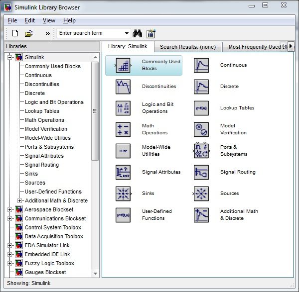
- The Library Browser contains various toolboxes in left side and corresponding utilities and blocks on the right side
To start creating a model go to File –> New or alternatively Ctrl+N. A Work space / Model window will pop up as shown below :

This is the place where you work on with. Creating models and simulating it, all this will be done here. The user just have to click and drag appropriate blocks from the library browser on to the Work space/Model window.
Creating a Model
Here i’m going to create a simple model of integrating a sine wave and display both the input sine wave and the integral form. To create this model we need,
- A sine wave signal source
- Integrator
- A Multiplexer, as i need to display the 2 signals in the Display screen. Note that the display screen called ‘scope’ has only 1 channel. So either to show 2 signals we have to use a mux or we have to use 2 screen blocks
- A display screen
Charting down all the needed components is good practice when it comes to designing of higher models
STEP 1 : Selecting Blocks
- For a sine wave sources
Simulink –>Sources –> Select sine wave from the list
- For Integrator
Simulink –>Continuous–>Select integrator from the block list
- For Multiplexer
Simulink –>Signal routing –> Select Mux from the list
- For Display
Simulink –>Sink –> Scope
Don’t worry if you don’t know where your component is. There is a Search bar provided in the library browser where you can type your component and search for it.
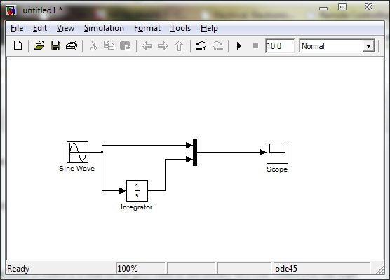
STEP 2: Block Creation & Making Connections
Select and drag all components to the model window and make connections:
- For making connections first select the input port and ‘+’ symbol will appear and drag the cursor to the output port ‘>’ symbol on the block. ( TIP: For making connections quicker select the input port hold Ctrl key & then click on to the output )
NOTE:
- You can change the attributes of the block like foreground / background color etc by right clicking and selecting the appropriate change.
- You can change the block parameters like gain value etc by double clicking on the appropriate item and changing the value. For eg: If in the above problem we can generate a discrete source of sine wave by changing time based to sample based.
STEP 3: Running Simulation
As the connections are made now your model is ready for running. Click on play button ![]() in the model window. Alternatively Ctrl+T or Simulation –>Start in the model window can be used to run the simulation model.
in the model window. Alternatively Ctrl+T or Simulation –>Start in the model window can be used to run the simulation model.
To view the result double click on the Scope block which is our display screen.
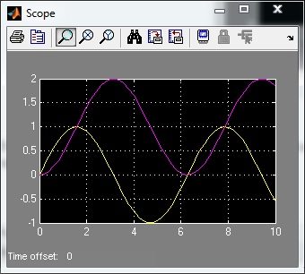
OUTPUT :

You can change the attributes of the axis by right click and specifying the axes properties. You can also auto scale the axes for a better view of the output.
NOTE:
- You may have noticed the output amplitude is 1. Its because by default the signal source amplitude is specified as 1. You can change the attributes of the blocks by double clicking on each one.
Simulation Control
Suppose if we want to control the simulation it can be managed by configuration parameters. Main parameters are start time, stop time, Solver type and methods.
For eg: We can decide whether integration is to be fixed step or variable step. If we are using Fixed Step we have to define the step size.
In the model window go to
Simulation–>Configuration Parameters. or alternatively press Ctrl+E.

STEP -4: Save the Model
To save the model
File –> Save As which is in the tool bar of model window.
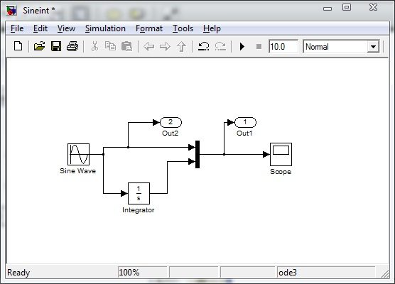
- Sometime if we wish to save the model in the MATLAB workspace and use MATLAB plot commands to display the data in the model. We have to use a Out block to represent the data we wish to plot. Here I’m going to plot both the input and its integrated form. So i have to use 2 out blocks as shown below
To use Out block
Simulink –>Sink –>Out
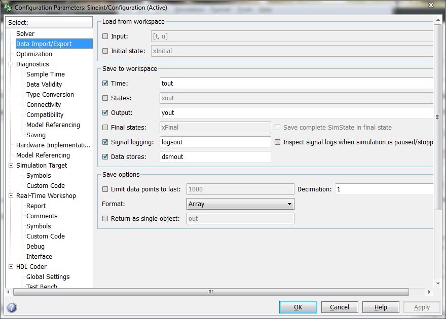
Now to see where our output gets stored and what variables are used open Configuration Parameters ( Ctrl+ E )
Go to Data Import/Export in it we can see there as time is stored as ‘tout’ and output stored as ‘yout’
Now if you want to know about the active variables ( tout and yout here ) you can use whos command in MATLAB workspace.
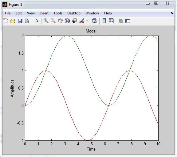
Now to plot the data in the workspace use plot commands.
plot(tout,yout);
xlabel('Time');
ylabel('Amplitude');
title('Model');


nice