
Contents
Here I’m going to show you how signals can be generated in MATLAB. If you are a newbie in this field, have a look at our MATLAB tutorials to get familiar with it.
Plotting of Discrete and Continuous signal
The 2 main functions for plotting are
- plot() function – For plotting Continuous signal
- stem() function – For plotting Discrete signal
stem() – 2-D plot function for plotting discrete sequence of data
SYNTAX :
- stem(y) – Plots the data sequence y specified equally spaced along x axis
- stem(x,y) – Plots x versus the columns of y. x and y must be of same size
- stem(…,’fill’) – If we want to fill the marker at the end of stem
- stem(…,LineSpec) – For specifying line style and color
For details about plot(), please go to this page.
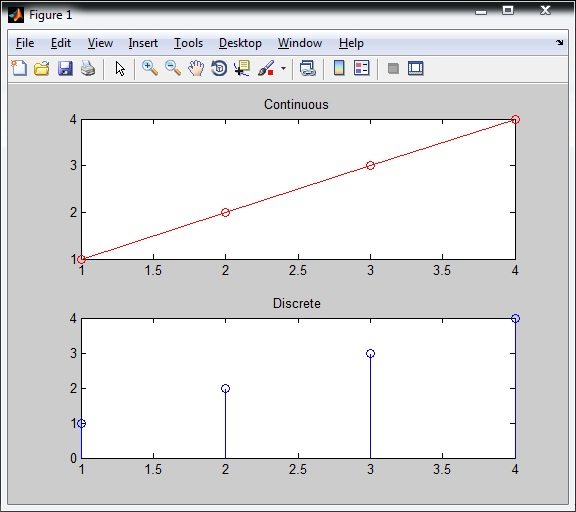
Plotting an Array of Data
x=[1 2 3 4];
subplot(2,1,1); # refer NOTE
plot(x,'ro-');
title('Continuous');
subplot(2,1,2);
stem(x);
title('Discrete');
Output :
NOTE:
- subplot() – is a function MATLAB which allows us to draw 2 or more graphs simultaneously on a single figure window. The function breaks the figure into matrix specified by user and selects the corresponding axes for the current plot SYNTAX : subplot(m,n,p) – Divides the figure window into m x n matrix of small axes and selects the pth axes object for the current plot. eg : subplot (2,2,1) – divides the figure into a 2 x 2 matrix (4 equal parts) and selects 1st axes object.
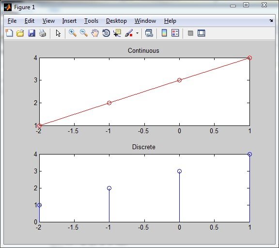
- The important point to be noted while dealing with the array data is MATLAB index starts with 1, ie by default MATLAB always assumes x(1) as the first element of the array [in above eg: x(1)=1]. So if we have to change the time index we have to define the range.
eg:
x=[1 2 3 4];
dtx=-2:1; #defining discrete time for x, from -2 to 1
subplot(2,1,1);
plot(dtx,x,'ro-');
title('Continuous');
subplot(2,1,2);
stem(dtx,x);
title('Discrete');
Output :
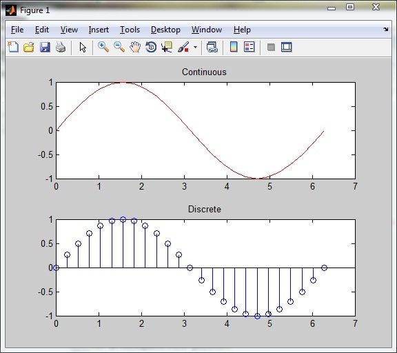
Plotting a Function
Now lets plot a function continuously and discretely. I’m going to plot a sine function
x=linspace(0,2*pi,25); # 0 to 2pi is divided in 25 equidistant points
y=sin(x);
subplot(2,1,1);
plot(x,y,'r');
title('Continuous');
subplot(2,1,2);
stem(x,y);
title('Discrete');
Output :
Some Basic Test Signals
While generating signals its range has to be specified it can be done in 2 ways
- Directly specifying range value
eg: -5:5 ; 0:10 etc - Can be specified during the runtime of the program using the input function in MATLAB.
SYNTAX :
input( ‘string’); # returns the input value
Now lets generate same basic test signals.
I. Impulse function
Impulse function given by
∂ (t) = { 1 for t=0 ; 0 otherwise }
n1=input('Lower limit')
n2=input('Upper limit')
x=n1:n2;
y=[x==0];
stem(x,y,);
Output :
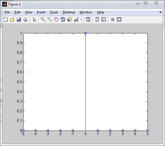
n1=-5 ; n2=5
II. Unit Step Signal
u(t)={ 1 for t >=0 ; 0 for t< 0 }
Discrete
n1=input('Enter the lower limit');
n2=input('Enter the upper limit');
n=n1:n2;
x=[n>=0];
stem(n,x);
title('Unit Step Signal - Discrete');
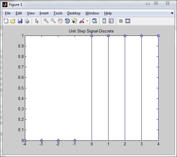
n1= -4 ; n2 = 4
Continuous
n=input('Enter the upper limit');
t=0:n;
x=[t>=0];
plot(t,x);
title('Continuous');
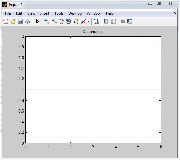
n = 6
III. Unit Ramp Signal
r(t)={ t for t >= 0 ; 0 for t <0 }
Recall that ramp signal r(t)=t*u(t) where u(t) is unit step signal
n1=input('Enter lower limit');
n2=input('Enter upper limit');
n=n1:n2;
x=n.*[n>=0];
subplot(2,1,1);
plot(n,x,'r');
title('Continuous');
subplot(2,1,2);
stem(n,x,'b');
title('Discrete');
Output:
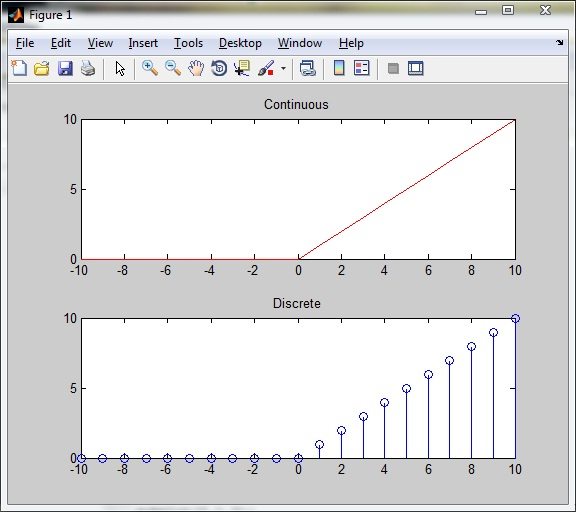
n1=-10 ; n2=10
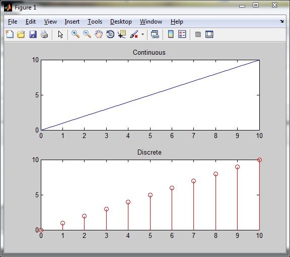
Shortcut method for Generating Ramp Signal
n=input('Enter the upper limit')
t=0:n;
subplot(2,1,1);
plot(t,t);
title('Continuous');
subplot(2,1,2);
stem(t,t);
title('Discrete');
Output :
IV. Unit Exponential signal
x(t)= eat
n1=input('Enter lower limit');
n2=input('Enter upper limit');
t=n1 : n2;
a=input('Enter the value for a');
y=exp(a*t);  # exp() function in matlab SYNTAX : exp(a)n- returns the exponential factor of a
subplot(2,1,1);
plot(t,y,'r');
title('Continuous');
subplot(2,1,2);
stem(t,y,'b');
title('Discrete');
Output :
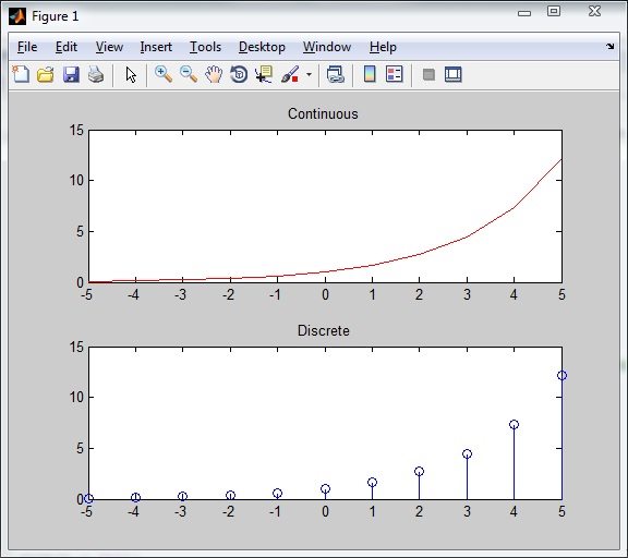
n1 = -5 ; n2= 5 ; a = 0.5
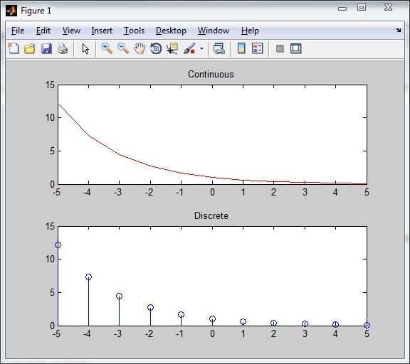
n1 = -5 ; n2 = 5 ; a = -0.5